Header image is D700 noise tests by Carl Jones used under license CC BY-NC
Following up on my previous post, I wanted to go into some detail on how I modelled NHL goalie performance this year.
If you just want to get your hands on the code, you can find it here. Likewise I have uploaded data so you can replicate what I did.
Introduction
The background story here is that I went a little too far in preparation for my hockey pool last year. See this, this, this, and for good measure, this. I built some models, predicted some things, and won. That’s the idea!
For this year I replicated my methodology from last year, somewhat more casually. What I did a lot differently was calculate my own goalie projections.
Predicting goaltender performance is hard. Goalies are subject to the whims of the gods and the players in front of them, whichever is least merciful. Most of our goalie stats capture team play as much as goalie ability. Goalies seem to vary year-over-year in how well they play. Add in a healthy dose of randomness (and uncertainty between randomness and performance variance), and our stats are all over the place.
Digging into my toolbox of handy modelling strategies, I chose to go for an old favourite: gradiant tree boosting.
Overview of Boosted Tree Models
Tree models are really not as hard as Wikipedia makes them look. Unless you like math, in which case they’re exactly as easy as Wikipedia makes them look.

This is the most complicated equation I will use.
maths from Sean MacEntee used under licence CC BY
Start with one decision tree. A single tree is just a model where you split the population into two (sometimes more, depending on the type of tree) groups based on one variable, and then split either of the resulting nodes on that or another variable, and so forth. Have you ever played the game 20 questions? If you’ve taken enough roadtrips, you might have. One person thinks of something, the other person has 20 questions to guess what it is. As this guide says, “TIP: With each question try to cut the number of possibilities in half.” If you can play 20 questions, you can build a tree model.
So say you have one tree. How do you boost it? You build another tree! Imagine you ran out of 20 questions and there were still cases you could not account for. Start with your first tree as the baseline, and build a second tree off of it. In practice we generally do not let the first tree have 20 splitters of depth, and we only slightly accept its predictions (the extent to which we do so is called the learning rate.
The concept doesn’t get any more complicated than that, although some of the details might.
So you’re gonna use tree models…

Okay, so why this type of model over your standard linear and logistic regressions, or something like a neural network? Maybe I’ve convinced you that it could work, but I’ve offered no explanation of why it should ever work better than anything else.
One of the main benefits is laziness. Really. These trees are exceptional at finding non-linear relationships, and for finding interactions between variables. This happens because they can split a node, changing it from a leaf node to a branch node, at any point they want, whatever point improves their performance the most. Given enough depth or trees, we can fit any high dimensional relationship. Even though each split is like a yes/no question, given enough of them we can fit a linear relationship, or a quadratic relationship, or a complex interaction of several variables.
Getting your data
Maybe it’s a topic for a future post, but I have a long-standing habit of scraping. Thank you hockey-reference.com for your well-organized data! You can find my versions of it in my data repo.
Choosing the feature space
There are somewhat three types of inputs I use to predict each target variable (e.g. games played, wins, goals against average):
- The target’s own lag and recent average. The best predictor of future production is past production.
- The league average (weighted), since some factors tend to move across the league (and are also messed up by lockouts).
- Other variables’ lags or averages. In particular, I expect past wins will predict future games played.
Specifically, here’s how I set this up, after building the variables:
def define_predictors(stat, extra_predictors):
    """Define the combined predictor set."""
    predictors = list(set(['age',
                           stat + '_lag',
                           stat + '_wt_avg',
                           stat + '_lag2',
                           stat + '_lg_wt_avg',
                           stat + '_lg_wt_delta']))
    if stat in extra_predictors:
        predictors = list(set(predictors + extra_predictors[stat]))

    return predictors

extra_predictors = {'GP': ['W_lag', 'GAA_lag', 'SV%_lag'],
                    'W_per_GP': ['W_lag', 'GP_lag'],
                    'SO_per_GP': ['W_lag', 'GP_lag'],
                    'SV_per_GP': ['W_lag', 'GP_lag', 'GP_avg', 'SV_per_GP_wt_avg'],
                    'GAA': ['GP_lag', 'GP_avg', 'GAA_wt_avg'],
                    'SV%': ['GP_lag', 'GP_avg', 'SV%_wt_avg']}

for stat in ['GP', 'W_per_GP', 'SO_per_GP', 'GAA', 'SV%', 'SV_per_GP']:
    predictors = define_predictors(stat, extra_predictors)

    # ... Do stuff
Note that by including the lag and the league average lag, I am implicitly including the difference between those two lags. Meaning, regardless of whether what really matters is the league average or the goalie’s performance relative to league average, the model can identify and fit either relationship. This is a benefit of the tree structure, which can find deep non-parametric interactions automatically.
Much like skater predictions, for several variables I predict them per games played, and separately predict games played, and then multiplying them. I think this is more necessary than otherwise because of lockouts, and injuries may be largely stochastic. But perhaps the biggest benefit of this decision is that the separability allows an end user to substitute the games played estimate with a more likely one. This is especially relevant for goalies who have switched teams and will have a much bigger or smaller role, for which my model knows nothing about that. It also means my games played and wins estimates are consistent with each other: doing it this way means it is impossible to predict more shutouts than wins.
Building it in Python with scikit-learn
Running these in scikit-learn is very easy. I use sklearn.ensemble.GradientBoostingRegressor to fit one of these, and sklearn.grid_search.GridSearchCV to run a grid search across the parameters, while using cross validation.
Grid search means there are a number of ways to parameterize the tree model, and you can search a number of combinations to find one that is best, for some definition of best. In more serious applications I closely examine which parameters work better, to understand which relationships are being identified in the model. But here I’m just goofing around.
from sklearn.ensemble import GradientBoostingRegressor
from sklearn.grid_search import GridSearchCV

def build_model(X_train, y_train, cv=5):
    """Perform a GradientBoostingRegressor grid search and return the winner."""

    # Note to self: Use subsample for stochastic gradiant boosting, next time
    param_grid = {'n_estimators': [50, 100, 200],
                  'max_depth': [2, 3, 4],
                  'min_samples_split': [100, 200, 300, 500],
                  'min_samples_leaf': [5, 10, 20, 50],
                  'learning_rate': [0.01, 0.1],
                  'loss': ['huber']}

    grid_search = GridSearchCV(GradientBoostingRegressor(),
                               param_grid=param_grid,
                               cv=cv).fit(X_train, y_train)

    return grid_search.best_estimator_
What these parameters mean:
- n_estimators: How many trees to build (on top of each other). This determines how complicated your interactions can get, with the downside of more trees being more potential overfit
- max_depth: How deep any one tree can get. This is one way to stop the model from overfitting on really specific relationships that will not extrapolate
- min_samples_split: How large a node has to be for the model to branch off of it
- min_samples_leaf: How large a leaf node has to be
- learning_rate: The multiplier on each tree, deciding how much we trust that specific tree
- loss: This is what your model will try to minimize. I was worried that least squares might be too sensitive to weird outliers
There are other parameters available, but these are the ones I used and took a quick look at.
How to interpret your results
One of the complaints about complicated models is that they aren’t easily interpretable. We do need to be able to understand what our model is saying and how it got there, because there are so many ways to accidentally build a model that will not extrapolate out-of-time in live data.
I always review my model performance versus model complexity, and the resulting influence of each variable.
In the example here, for the games played model, we can see that performance continues to improve on both the training and test data as we add more trees (much like golf, lower is better, and things get boring pretty quickly), but that while the training data continues to fit better, eventually the test data flattens out. It can even start to perform worse if the training data is terribly overfit.
We can also see that league average games played is the most important variable (caveat on that below), followed by age, and then the goalie’s career average and their prior season.
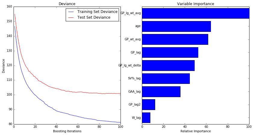
Importance here is a bit fuzzy, since it is calculated based on how the loss metric changed at each split, summed for each variable (scaled to the most important being 100). This can vary immensely if two variables are highly correlated, such that either could have been used.
That’s one big reason of why I prefer partial dependence plots (PDPs). These show me not only a scale of how relative changes in each variable change our prediction, but they also show me the shape of those relationships. This is key for seeing how your model will react to different inputs, and whether it is overfit or there is some other data mistake. If you were to apply the values of your variable across all of the rows in your dataset (e.g. multiply the dataset) and look at the average score by each value, you get these. They’re scaled such that each one averages 0.
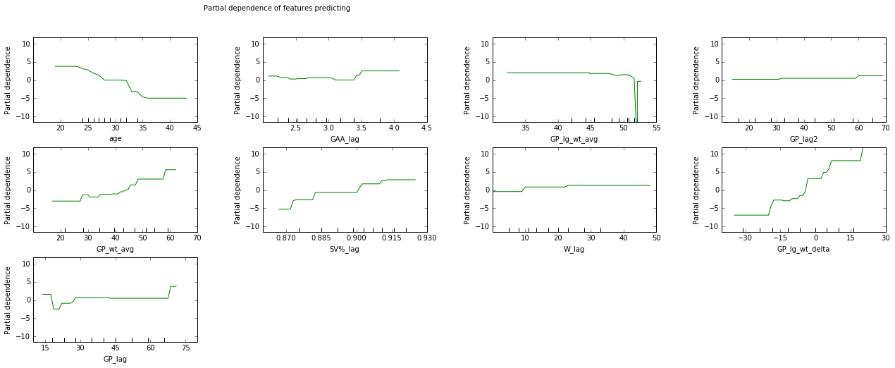
We can see that the league average is actually not a great variable here, and might just be overfitting on one weird case (the year before a lockout?). But other variables are sensible. Games played, GP relative to league average, save percentage, and age are all important, while the others have minor effects. Note that monotonicity is not guaranteed (potential movie title for the sequel to Safety Not Guaranteed? I’ll talk to Colin Trevorrow), and evidence of a too discontinuous relationship could suggest overfit.
Wrapping up
You can check out my prior post for some of the key results, so I won’t rehash them here. Goalies are tough to predict, and I took the casual lazy way of making these predictions, so even I don’t use them entirely on their own.
One of the cool results was figuring out how predictable different stats were. This helped me decide how much to weight each category in my draft, much like I do for skaters. GAA was the most predictable (in a rank-ordering way), which I suppose makes sense since it’s basically a team stat and teams vary less than goalies do.
After all was said and done, I drafted Brian Elliot and Craig Anderson in my hockey pool. Let’s hope Ottawa doesn’t read my old post and think that Andrew Hammond is the best goalie in hockey, and that Craig Anderson fights my age curve!